Volume 1, Issue 1
Article Type: Research Article

Chronic obstructive pulmonary disease prediction using deep convolutional network

Shahran Rahman Alve^*; Muhammad Zawad Mahmud; Samiha Islam; Mohammad Monirujjaman Khan

¹Department of Electrical and Computer Engineering, North South University, Bangladesh.

*Corresponding author:  Shahran Rahman Alve
Department of Electrical and Computer Engineering, North South University, Bashundhara R/A, Dhaka 1229, Bangladesh
Email ID: shahran.alve@northsouth.edu

Received: Feb 17, 2025
Accepted: Mar 17, 2025
Published Online: Mar 24, 2025
Journal: Biomedical Engineering: Open Access
Copyright: Alve SR et al. © All rights are reserved

Citation: Alve SR, Mahmed MZ, Islam S, Khan MM. Chronic obstructive pulmonary disease prediction using deep convolutional network. Biomed Eng Open Access. 2025; 1(1): 1003.

Introduction

The clinical benefits area is different, and it is one of the most important ways to tell different projects apart. It is one of the most important and important areas where people want to spend their money on the best level of finding, therapy, and first-class organizations. Different clinical equipment’s pictures and sounds may have different purposes because of their partiality, clarity, and many different designs. They may be given to a wide range of people after being checked by different translators or experts [1]. In the not-too-distant past, we had to rely on human knowledge, limits, and breadth of abilities to interpret and understand the huge amount of clinical data made by different machines and automatic assembly types. Continuous Obstructive Pneumonic Disorder (COPD) is a group of lung infections that make it hard to relax because they block the flow of air through the lungs by making the airways narrow. The lungs can’t get enough oxygen and give off carbon dioxide, which is irritating. Emphysema and chronic bronchitis are the two main diseases that lead to COPD [2]. People with COPD often have both of these problems at the same time, and they can get worse quickly. When you have bronchitis, you need to learn how to fly with limited fuel [3]. COPD is known to be caused by smoking, having a genetic disorder [4,] air pollution, and other things. COPD has not yet been found early or completely. This is still a work in progress that has not reached 100% accuracy.

Generally utilized procedures by clinical experts right now are [5]:

• Respiratory muscles tests: In these assessments, we check to see if the person’s lungs work well and give off enough oxygen when they relax. Spirometry is the most well-known test for this. In Spirometry, the person breathes into a machine called a “Spirometer,” which measures how often air the person breathed in.

• Chest X-ray: A chest X-ray can find a number of respiratory illnesses, but Emphysema is the most common one. COPD is often caused by emphysema.

• CT extract: CT Sweep isn’t used very often, but it is used in crazy situations where it’s impossible to identify someone using normal methods. A CT report can show whether or not a patient with COPD needs any kind of routine treatment.

• Blood vessel venous blood test: This test measures how much oxygen rises in a person’s blood when they relax.

Impediments of as of now utilized strategies:

• Spirometry can’t be done on people who have serious heart problems or who have just had heart surgery.

• Some of the side effects that often happen after the tests are feeling out of breath, sick, and confused.

• Both CT Sweeps and X-Beams put patients at risk because they expose them to radiation.

With so many limits and research methods based on manmade cognizance, many studies have shown that intelligence and meaningful learning cost estimates were broken down, looked at, and used to see if they could help give better and more accurate results and help professionals with COPD. With a real calculation, you can find out where COPD is in a picture or by listening to the respiratory organs. The “connected job” segment shows how robotization and real systems can help find out what’s wrong with a person’s lungs. Real-world technologies like the Breath Noticing Structure [6] suggest a quick breath inspection device that could be used to find COPD. A classifier based on ANN and backpropagation-based Multi-layer Perceptron computation was studied to predict the fundamental respiratory sound event in patients with certain respiratory diseases, most often asthma and COPD [7]. Because ANN is not a linear system, its results are better than those of the more common gathering or backsliding methods. In a similar way, more evaluation can be done by fixing the classifier’s flaws or using explicit computer-based intelligence methods like substantial learning. At the top event level, precision and audit were 77.1% and 78.0%, respectively, and 83.9% and 83.2% for other events. The average rate of a machine doing something is 81.0%. People have come up with a simplified framework for chronic illness that gives a stage for productive discovery and consistent evaluation of the health status of COPD-contaminated patients [8]. A machine is being put together so that doctors can see a patient’s condition in real time. On a customized, up-to-date partner, a hybridized classifier was made with a ml estimate like SVM, a sporadic forest area, and a predicate-based way to manage a more spectacular request with the goal of grouping a COPD series early and consistently. At 94%, there is still doubt about how good the plan is. A PC-based method for handling typically translated stethoscope-recorded respiratory sounds has also been shown [9]. This method has many possible uses, such as telemedicine and self-screening. One test device is used to record three types of breathing sounds from 60 people. A major model of Convolutional Mind Associations is shown next. It has six layers of convolution, three layers of max-pooling, and three layers that are all connected. Time-repeat change was used to get 60 Log-scaled Mel-Repeats. Extraordinary characteristics were taken from the dataset frame by frame and split into 23 nonstop housings as model commitments. Lastly, the model was tested with a new set of data from 12 people and survey results from 5 respiratory experts to see how accurate it was. Aykanat et al. (2017) suggested a simple and useful electronic stethoscope that can be used on any unit to record lung sounds on a screen. With this device, 17,930 lung sounds from 1,630 participants were recorded [10]. The audit used two types of AI calculations: Mel repeat cepstral coefficient features in Convolutional Mind Association (CNN) and SVM nearby spectrogram images. Most people agree that using MFCC convenience for an SVM calculation is a good way to make a sound request, so the sponsors used its tests to check how well the CNN estimation execution worked. Each CNN and SVM calculation produced four useful lists for the request of respiratory sound: rale, rhonchus, and the standard representation of talk; a single list of respiratory talk design; and a layout of the sound type of each sound structure. Exploratory precision disclosures were 86% CNN, 86% SVM, 76% CNN, 75% SVM, 80% CNN, 80% SVM, and 62% CNN, 62% SVM. All of these were done on their own. So, it was found that both the CNN and SVM estimates did a great job with spectrogram image collection skills. If CNN and SVM have a lot of data, they can use the sounds of breathing to correctly detect and pre-select COPD. In the study, different enlistment abilities of the ANFIS, MANFIS, and CANFIS models were used to show spirometry results [11]. The ANFIS estimate gives more accurate confirmations than the mind network technique that was just used. This could be because ANFIS controls how the brain’s learning limits connect to the thinking limits of the cushioned determination system. As was already said, CANFIS is 97.5% more accurate with requests than ANFIS and MANFIS. Chamberlain et al. (2016) [12] focused on wheezes and snaps, which are the two most progressive lung sounds. Their calculations led to ROC curves with AUCs of 0.86 and 0.74 for wheezes and 0.74 for pops, respectively. In another evaluation, 155 models from the COPD disease dataset were separated into two groups: Class 1: COPD (55 models) and Class 2: Standard (100 models). The results of a two-mystery-layer MLNN system (95.33% accuracy) were better than those of a single-mysterylayer MLNN system. In a survey that was set up to test data [12], a feed-forward NN design with a hidden layer based on the log sigmoid trade feature was used. This connection was made up of a lot of simple, layer-based units that worked like neurons. The association testing was finished, and because of the mistake, the results were turned around. Controlled learning is often used in networks in the cerebrum that work for a long time. RBF associations are a good way to show nonlinear data because they can be done in a single step, unlike Different Layer Perceptron, which has to be done over and over again. Relationships with more people grow quickly. To find the solution for the relationship, the results of the mystery layer are added together to make a data vector, which is then broken down using the best answer for the result layer. The piles are made in a straight line, following a set of rules. Computer-based intelligence methods may be able to help find COPD worsening early [13]. Using an escalation gauge could lower the risk of things going wrong that could be life-threatening and cut down on the high costs that come with having COPD. Extreme increases are one of the main reasons why people with chronic obstructive pulmonary disease have a lower quality of life and end up in the hospital (COPD). The dispersed model may be able to find early signs of COPD worsening 4.4 days before they show up. There was a decision tree for classifying woodlands, and it was approved by using recorded data for updated intensification assumptions based on secondary effects. Estimates based on deep learning, like CNN and LSTMS, are really standing out to the point where they are seen as important learning frameworks [14]. Using large datasets of respiratory sound noises and spectrogram images, we can design important brain networks without using pain-based features to detect COPD in people who are very aware and expressive. The main benefit of using this motorized COPD disclosure method is that model outputs are consistent (because a model predicts similar features each time on the same image), there is a high level of responsiveness, results change over time, and there is a high level of expressivity. Furthermore, since a calculation has a few practical centers, the reactivity and exactness may be designed to match diverse clinical condition standards, comparable to high responsiveness for a screening system. Standard ways to find out if someone has COPD were a Pulmonary Function Test or a simulated knowledge-based structure, which required images to be handled with as much care as possible to find the disease. Coming to the crisis center and making the basic finding by chest result or xshaft in case of any respiratory wretchedness scenario, for example, a coronary letdown or asthma attack, is tedious, pricey, and risky. Similarly, the motorized reenacted knowledge structures for image-based acknowledgement need establishing the model on massive quantities of amazing HD images of x-bar, which is seeking to obtain each time. In view of everything, there is an imperative for a more uncomplicated moreover, less resource concentrated structure, which may enable clinical consideration providers promptly establish the fundamental discovery. The structure we presented is a system that identifies COPD by listening to respiratory noises. The sound produced by the body’s internal organs is rather astonishing in the event of a cardiac episode, asthma, COPD, and so on. Motorized detecting such noises to bunch in the event that a person is weak due to COPD is an overly skilled, self-upsetting operation for both the individual and the trained expert. The framework for the declared region of COPD might be included by the professionals. Alternatively, the future growth of this system includes collaborating with smart gadgets and microphones to continually record people’s noises and so anticipate the possibility of an instance of COPD.

The current work proposes a novel CNN architecture for improving speed COPD detection accuracy. To properly identify COPD, the proposed approach consumes fewer processing resources. The remainder of this work is divided into the following sections: The approach and materials are discussed in Section 2. Section 3 discusses the results, and Section 4 wraps up the conclusion.

Methods and materials

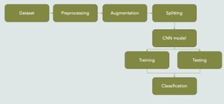
The data was taken from publicly available online sources. After separating the training and test sets, the next step is to import and extract pictures and annotations from raw datasets. Then, preprocessing and enhancement methods are used. In the next section, we’ll show you how to create hyperparameters, use regularization, and apply an optimization strategy. Finally, there are estimations for system training and performance. The CNN model, developed by Google Colab, is used to distinguish between normal and aberrant sound.

Dataset description

This study was based on the Respiratory Sound Database dataset [15], which is freely available. The Respiratory Sound Data set was made by two examination groups in Portugal and Greece. It incorporates 920 clarified accounts of fluctuating length 10s to 90s. These accounts were taken from 126 patients. There is a sum of 5.5 long stretches of accounts containing 6898 respiratory cycles 1864 contain snaps, 886 contain wheezes and 506 contain the two pops and wheezes. The information incorporates both clean respiratory sounds as well as boisterous accounts that reproduce genuine circumstances. The patients range all age gatherings youngsters, grown-ups and the old.

Data preprocessing: The data set was full of mistakes and was not well organized. To make the data more comparable, we used the Python tool Librosa to make sure that each sound report was 20 seconds long. For the part extraction, we chose five characteristics. Mel-Repeat Cepstral Characteristics were coefficients, which were not fully determined by the waveform/ power spectrogram, the ConstantQ Chromagram, or the chroma cents. A mel-repeat cepstrum is made up of MFCCs, which are coefficients. A MFC is a representation of a sound’s transient power range that takes into account straight cosine changes in a log power spectrogram on a non-direct mel size of repetition. These qualities deal with phonemes because they show how the vocal package is doing. So, MFCC is a confusing thing to think about when evaluating respiratory sounds. To make the Mel-Spectrogram, we step through pneumatic pressure tests over time, map it from time space to repeat space using the quick Fourier Change, and convert the frequency to a Mel scale and the collection viewpoint to the adequacy. It is the range of a sound’s power as it changes. As mentioned above, “pitch class profiles” can also be inferred from chroma-based qualities. These are important areas of strength for a wide range of components used to evaluate music whose pitches can be asked for. Chroma plays an unusual role in our client’s case because the pitch of the breathing sounds changes in a clear way.

Because CENS characteristics are sensitive to components, tone, and articulation, they are often employed in sound organization and recovery applications. To ensure uniformity among features, we assigned the “n” value of 40 to all components.

Data augmentation: Since the number of COPD tests was often almost the same as the number of non-COPD tests, we used different sound extension techniques on the guides to increase the number of non-COPD tests. Keras and Tensorflow are used to build our CNN. It is a progressive model with a Data Layer, Convolution 2D layers, DropOut Layers, MaxPooling2D Layers, and a Thick Layer. ID is the most important part of a convolution layer. It works by dragging a channel window across the data and making a part map of the moving structures as the window moves. A component map ages through a process called “convolution.” Each convolutional layer has a MaxPooling2D pooling layer, and the final layer is a GlobalAveragePooling2D pooling layer. The pooling layer’s job is to reduce the number of dimensions in the model. It does this by working on the limits and making suggestions for fewer estimate needs. This cuts down on the time it takes to plan and the chance of overfitting. Maxpooling and the Overall Typical Pooling type use the best and average window sizes for each window to handle our thick result layer. The number of different ways to play the character is chosen with these two points in mind. Softmax is where the result layer starts. As a possibility, Softmax raises the number of results to a very high level.

Block diagram

Figure 1 depicts the research method as a system diagram.

The channel limit does not specify how many centers are allowed in each. The size of the single layer gradually increases from 16, 32, 64, to 128, while the piece size restriction depicts the part window size, which is two, obtaining a 2 2 channel matrix. The possible advantages of data form would be (40, 862, 1), with 40 being the number of MFCCs, 862 being the number of edges taking padding into consideration, and 1 being the mono sound development. The components are then sent via the Convolution2D layer (16 channels, part size: 2, relu) before being passed to the MaxPooling2D layer. To prevent overfitting the data, we used a dropout rate of 20%. Following the dropout, the data is sent to a Convolution layer (32 channels, part size:2, relu), which then sends it to a MaxPooling2D layer (Pooling size: 2). There is, without a doubt, a Convolution2D layer (64 channels, bit size: 2, relu), a MaxPooling2D layer (Pooling size: 2), and a 20% dropout following a 20% dropout. The data is then processed by a Convolution2D layer (32 channels, part size:2, relu), a MaxPooling2D layer (pooling size: 2), and a dropout layer (20%). ReLu is the start-up capacity utilized for the duration of activation map from the convolutional layer. Finally, we send the excess data to the GlobalAveragePooling2D layer (128) to fix the result and then transfer it to a thick layer to cluster it into two outcomes, explicit COPD and non-COPD. The suggested method’s system architecture is shown in Figure 2.

When compared to the picture inputs, it can be noticed that the sound data sources all around have a larger amount of noise. We used the Adam improvement estimator to smooth out our model since it is computationally powerful, takes less memory storage, and provides improved performance for disordered data values. Adam is a combination of stochastic slant fall and RMSprop calculation, which delivers better association weight upgrade reasoning, making the process of hyper limit tweaking more plausible [16]. When compared to other current optima’s such as RMSprop, SGD, ADAGrad, and NAdam, this algorithm provides a faster blend with smoothed-out execution constraints.

Proposed system

Convolutional layers, ReLu, and Dropout were used in this network’s convolution block. The convolutional layer behaves in the same way as the max-pooling layers. The SoftMax function is located in the last layer. A 2D convolutional layer moves K convolutional filters (kernels) of size (M X N) over the input images, calculating the dot product of the weights (kernel weights) and the input. The vertical and horizontal movement of the filters across the image is referred to as a “stride.” Padding (P) of the original images may be added before sliding the filters to keep information at the borders. Dropout (D) is a fundamental neural network overfitting avoidance strategy. These kernels are used to discover features, and they range from early-layer kernels that merely look for low-level features like edges, lines, and blobs to more complicated kernels that look for more nuanced attributes. For the convolutional network, we used the following parameters: filter = 64, 128 and 128, kernel (M*N) = 3*3, 3*3, Stride = [1, 1, 1], Padding = same, Dropout = 0.2. For dropout layers, a dropout rate of 20% was determined to be optimal. Every neural layer is followed by a non-saturated activating function known as ReLU, which significantly decreases training time when compared to other activation functions. When x is positive, the output equals the input, and 0 for all other values, hence the ReLU model is given as a function of x. Maximum pooling is a kind of downsampling that achieves spatial invariance by splitting the whole image into small rectangles (3x3 in the recommended structure) that travel across the image in a predetermined step (3x3) and then evaluating only the maximum value of the four components. The pooling layer of the network reduces the number of parameters and, as a result, the number of computations. The suggested CNN design is shown in Figure 3.

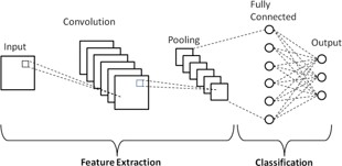
The network architecture is shown in Figure 3, which contains an input, three convolutional units, a classification unit, and an output. During the first critical block, block 1, a convolution layer produces an output that is twice as large as the input. 3*3*64 filtering with phase=1 and padding equal to the cost of the first convolution layer is used to convolve the first convolution layer. Following convolution, the convolutional layer reacts with a 20% dropout to the rectified unit (ReLU) activation phase and the dropout layer. This block also has a max-pooling layer, which produces an output that is twice as long as the input. Unit 1’s output is used as an input in Block 2, which convolves it with 3*3*128 filters with stride=1 and padding=1, although no dropout layer is used. We used batch normalization instead of a dropout layer, which allows each layer of the network to train separately. The response of the convolutional layer is based on the maximum pooling layer and the rectified linear unit (ReLU) activation layer. This block creates an output that is twice the size of the input after max-pooling the convolution layer’s response. The third block, convolution setup, is similar to Block 2, with the exception that we used a 20% dropout this time. The maximum pooling layer and the rectified linear unit (ReLU) activation layer define the response of the convolutional layer. the same way as the max-pooling layers. The SoftMax function This block takes the result of block 2 as an input and provides an output that is twice the size of the input after max-pooling the convolution layer’s response. The output of this block is utilized as the input for the classification block that follows. The classification block is made up of four fully connected (FC) layers, the first of which shows the flattened output of the previous maxpooling layer to 8192 nodes. The second layer is dense with 128 nodes, while the third layer is likewise dense with 64 nodes. The final thick layer, which has the same number of hidden units as target classes, was generated using SoftMax.

Cross-validation

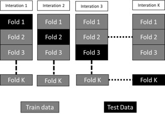
In this study, performance was evaluated using the crossvalidation method. We could gather additional data and draw meaningful conclusions regarding our technique and data. To begin, the whole data set is divided in half, with training images accounting for 90% of the data and test images accounting for 10%. We just used the train data for cross-validation. As shown in Figure 6, data is often divided into ten roughly equal sections, nine of which are utilized for training and one for validation. Because each segment has the same amount of data, cross-validation is achievable. In each cycle, nine randomly selected portions are used to train the model, while another piece is used to verify it. We segregated test data from production data from the beginning so that we could examine the model using photographs we weren’t aware of. The cross-validation method is shown in Figure 4.

Performance matrix

The system displayed real and expected values on a confusion matrix. The predicted outcomes of a classification model are represented by the confusion matrix. The precision, sensitivity, specificity, and accuracy numbers were calculated as follows [21,32]:

The phrase “True Positive” refers to the number of circumstances that are predicted to be positive but actually happen (TP). True Negative refers to the proportion of predicted negative conditions that are also true negatives (TN). A False Negative (FN) is a term for the number of predicted negative events that turn out to be true, also known as a type two mistake. The number of predicted positive instances that turn out to be negative is known as a “False Positive” (FP).

Result and analysis

We employed a bespoke CNN model in our suggested system. The data was used to both train and enhance the performance of the models using 10-fold cross-validation. Without cross-validation, the model’s training accuracy was 98% and its validation accuracy was 95.0%. After evaluation, the test’s accuracy was verified to be 96%. Cross-validation enhanced the model’s performance tenfold. After cross-validation, the test’s accuracy was 96.5%. Cross-validation was used to increase the model’s performance.

Best model accuracy and loss

Figures 5 and 6 show the training and validation accuracy graphs, as well as the training and validation loss graph.

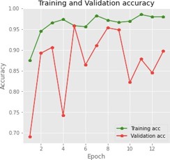
With a learning rate of 0.001, 64 sample sizes, and 14 epochs, the model was trained. The model’s performance improves with each epoch. In the first few epochs, the performance improves dramatically. Development slows after 5 epochs, and then after 6 epochs, efficiency hardly increases.

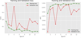
Figure 6 shows that the training accuracy was 98.0%, and the validation accuracy was 90.0%. As seen in Figure 6, validation loss is also bigger than training loss. This demonstrates that the model we described is not overfitted.

Other overfitted and low accuracy model accuracy and loss

Figures 7 show the training and validation accuracy graphs, as well as the training and validation loss graph.

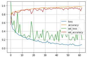
With a learning rate of 0.001, 64 sample sizes, and 60 epochs, the model was trained. In this case training accuracy and validation accuracy was 89 and 88% respectively. The accuracy was lower than CNN model. Figure 8 shows the Inception V3 model’s accuracy graph.

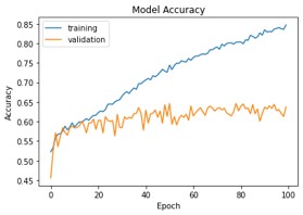
With a learning rate of 0.001, 64 sample sizes, and 100 epochs, the InceptionV3 was trained. In this case training accuracy and validation accuracy was 86 and 63% respectively. Also, with this model we received 86.90% test accuracy. But in this case training accuracy was much higher than validation accuracy which indicated that this model was fully overfitted.

Audio data visualization

With a 50ms FFT window size, spectrograms are produced. The spectrogram’s resulting bins are multiplied by the square of their frequency. Figure 9 shows the filtering diagram.

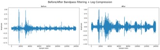
In this case, the amplitude square relation is ignored because ignoring it results in cleaner peaks. Transients are eliminated and the curve is smoothed out with a Guassian filter. On the smoothed curve, peak detection is next carried out. The timings of each peak’s left and right bases are then recorded, with respect to 80% of peak height. The dataset’s sound formatting image is depicted in Figure 10.

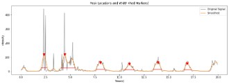
A reference for the beginning and end of a breathing cycle will be the left and right peak bases.A constant offset will be used for the left and right bases to estimate the beginning and end of the breathing cycle.Using the hand-annotated dataset, the values for will be determined by determining the value that minimizes the error between the predicted start and end of each breathing cycle. A multivariate optimization function is used to calculate the offset values. The objective function is the sum of the mean errors in the start/end times of the estimated and manually annotated cycles. Only the peaks that are the closest to the hand-annotated cycles will be compared because there are more detected peaks than cycles.

Model classification

While choosing the network architecture, several different architectures such as VGG-19, inceptionV3, EfficientNet and CNN are experimented with. CNN has performed the best among all the networks and we include the results based on that architecture. The history of the accuracy and loss of four experimented models is shown in Table 1.

Table 1: Comparison of different deep learning models.

The performance of the network was assessed using augmented audio, and the network’s growth was assessed using 10-fold cross-validation. The proposed network outperforms the competition with an overall accuracy of 96%. The model’s efficiency is 90% without cross-validation. Furthermore, the record-wise cross-validation strategy produced the best results for the 10-fold cross-validation method, with an average accuracy of 96%. Figure 7 shows how well a classification model works on a set of test data when the true values can be found.

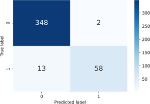
348 healthy audio and 58 COPD audio were properly predicted by the suggested CNN model. As a result, there were 406 accurate guesses in all. This model, on the other hand, projected that 2 healthy audios would become COPD audio. As a result, the total number of incorrect guesses in this scenario was 15.

Comparison of result

In this work, two methodologies were used to evaluate the suggested CNN model. Table 1 lists studies that have employed various types of CNN architectures. That study is compared to the proposed CNN model. The proposed model was 97% correct even without 10-fold cross-validation. This is a much superior system to the one we now have.

Table 2: Model’s result comparison.

This study achieved 96% accuracy using a custom CNN model, while Ref [18] achieved 93% accuracy using the CNN model. YOLO model ref [17] and [19], which also used VGG 19 techniques, had less accuracy than our suggested model.

Conclusion

In this paper, we have proposed a clear and less resource serious CNN-based significant learning assistive model, which can help clinical experts in recognizing COPD using respiratory sounds. In the coordinated preliminaries, we have used a Librosa man-made intelligence library feature like MFCC, MelSpectrogram, Chroma, Chroma (ConstantQ), and Chroma CENS to play out an unmistakable assessment of respiratory sounds [20] on the Dataset. Considering the coordinated assessments, it has been seen that as “mfcc” has given better precision in recognizing COPD stood out from any leftover Librosa man-made intelligence library features.

For the future expansion, we can loosen up its functionalities to help experts in distinguishing various diseases, for instance, probability of occasion of cardiovascular disappointment/cardiovascular breakdown considering the heart beats sounds, acknowledgment of Asthma considering lung sounds, etc. We can similarly work on the back-and-forth movement structure to perceive the earnestness of the contamination. We can in like manner apply different data extension techniques to deal with its show. Our system can be gotten together with a Breath Noticing Structure [31] to make the most well-known approach to perceiving COPD substantially clearer. Also, making this system attack protected and greater security safeguarded would be of most outrageous importance [22]. Realizing that the current framework could recognize COPD and non-COPD in most of circumstances, furthermore, we need to place our framework in different vehicles so we can concentrate on the aspiratory conditions progressively.

References

1. J Ahmed, S Vesal, F Durlak, R Kaergel, N Ravikumar, M RémyJardin, et al. COPD classification in CT images using a 3D convolutional neural network. In: Maier-Hein K, Palm C, eds. Bildverarbeitung für Die Medizin 2020—Informatik Aktuell. Wiesbaden: Springer Vieweg. 2020: 39–45.
2. G Altan, Y Kutlu, N Allahwardi. Deep learning on computerized analysis of chronic obstructive pulmonary disease. IEEE Journal of Biomedical and Health Informatics. 2019; 24: 1344–1350.
3. G Altan, Y Kutlu, AO Pekmezci, S Nural. Deep learning with 3Dsecond order difference plot on respiratory sounds. Biomedical Signal Processing and Control. 2018; 45: 58–69.
4. JL Amaral, AJ Lopes, JM Jansen, AC Faria, PL Melo. Machine learning algorithms and forced oscillation measurements applied to the automatic identification of chronic obstructive pulmonary disease. Computer Methods and Programs in Biomedicine. 2012; 105: 183–193.
5. M Asaithambi, SC Manoharan, S Subramanian. Classification of respiratory abnormalities using adaptive neuro-fuzzy inference system. In: Pan J-S, Chen S-M, Nguyen NT, eds. Intelligent Information and Database Systems. Berlin: Springer. 2012; 65–73.
6. M Aykanat, O Kılıç, B Kurt, S Saryal. Classification of lung sounds using convolutional neural networks. EURASIP Journal on Image and Video Processing. 2017; 2017: 65.
7. A Badnjevic, L Gurbeta, E Custovic. An expert diagnostic system to automatically identify asthma and chronic obstructive pulmonary disease in clinical settings. Scientific Reports. 2018; 8: 11645.
8. Z. Bai, Y. Li, M. Woźniak, M. Zhou, D. Li. 2020. DecomVQANet: decomposing visual question answering deep network via tensor decomposition and regression. Pattern Recognition 110:107538 DOI 10.1016/j.patcog.2020.107538.
9. CC Bellos, A Papadopoulos, R Rosso, DI Fotiadis. Identification of COPD patients’ health status using an intelligent system in the CHRONIOUS wearable platform. IEEE Journal of Biomedical and Health Informatics. 2014; 18: 731–738.
10. D Chamberlain, R Kodgule, D Ganelin, V Miglani, RR Fletcher. Application of semi-supervised deep learning to lung sound analysis. In: 38th Annual International Conference of the IEEE Engineering in Medicine and Biology Society (EMBC). Piscataway: IEEE. 2016: 804–807.
11. R Du, S Qi, J Feng, S Xia, Y Kang, W Qian, et al. Identification of COPD from multi-view snapshots of 3D lung airway tree via deep CNN. IEEE Access. 2020; 8: 38907–38919.
12. O Er, F Temurtas. A study on chronic obstructive pulmonary disease diagnosis using multilayer neural networks. Journal of Medical Systems. 2008; 32: 429–432.
13. MA Fernandez-Granero, D Sanchez-Morillo, A Leon-Jimenez. An artificial intelligence approach to early predict symptombased exacerbations of COPD. Biotechnology & Biotechnological Equipment. 2018; 32: 778–784.
14. KL Khatri, LS Tamil. Early detection of peak demand days of chronic respiratory diseases emergency department visits using artificial neural networks. IEEE Journal of Biomedical and Health Informatics. 2018; 22: 285–290.
15. ICBHI. ICBHI challenge. Available at https://bhichallenge.med.auth.gr/ICBHI_2017_ Challenge 2017.
16. KL Khatri, LS Tamil. Early detection of peak demand days of chronic respiratory diseases emergency department visits using artificial neural networks. IEEE Journal of Biomedical and Health Informatics. 2018; 22: 285–290.
17. Mahmud MZ, Reza MS, Alve SR, Islam S, Fahmid N. Advance transfer learning approach for identification of multiclass skin disease with LIME explainable AI technique. medRxiv. 2024.
18. Islam S, Mahmud MZ, Alve SR, Chowdhury MMU. Deep learning approach for enhancing oral squamous cell carcinoma with LIME explainable AI technique. arXiv preprint. 2024: arXiv: 2411.14184.
19. Alve SR. Deep learning and hybrid approaches for dynamic scene analysis, object detection, and motion tracking. arXiv preprint. 2024; arXiv: 2412.05331.
20. Y Liu, Y Lin, S Gao, H Zhang, Z Wang, Y Gao, et al. Respiratory sounds feature learning with deep convolutional neural networks. In: 2017 IEEE 15th International Conference on Dependable, Autonomic and Secure Computing, 15th International Conference on Pervasive Intelligence and Computing, 3rd International Conference on Big Data Intelligence and Computing and Cyber Science and Technology Congress (DASC/PiCom/ DataCom/CyberSciTech). Piscataway: IEEE. 2017: 170–177.
21. Mahmud MZ, Islam S, Alve SR, Pial AJ. Optimized IoT intrusion detection using machine learning technique. arXiv preprint. 2024; arXiv: 2412.02845.
22. S Patil, J Shashank, P Deepali. Enhanced privacy preservation using anonymization in IoT-enabled smart homes. In: Smart Intelligent Computing and Applications. Singapore: Springer. 2020: 439–454.
23. D Perna. Convolutional neural networks learning from respiratory data. In: 2018 IEEE International Conference on Bioinformatics and Biomedicine (BIBM). Madrid: IEEE. 2018: 2109–2113.
24. D Perna, A Tagarelli. Deep auscultation: predicting respiratory anomalies and diseases via recurrent neural networks. arXiv. 2018.
25. L Pham, I McLoughlin, H Phan, M Tran, T Nguyen, R Palaniappan. Robust deep learning framework for predicting respiratory anomalies and diseases. arXiv. 2020..
26. AV Radogna, N Fiore, MR Tumolo, V De Luca, LT De Paolis, R Guarino, et al. Exhaled breath monitoring during home ventilotherapy in COPD patients by a new distributed tele-medicine system. Journal of Ambient Intelligence and Humanized Computing. 2019; 5: 1–9.
27. BM Rocha, D Filos, L Mendes, G Serbes, S Ulukaya, YP Kahya, et al. An open access database for the evaluation of respiratory sound classification algorithms. Physiological Measurement. 2019; 40: 035001.
28. A Shaikh, S Patil. A survey on privacy enhanced role-based data aggregation via differential privacy. In: 2018 International Conference on Advances in Communication and Computing Technology. Piscataway: IEEE. 2018: 285–290.
29. J Weese, C Lorenz. Four challenges in medical image analysis from an industrial perspective. Medical Image Analysis. 2061; 33: 44–49.
30. R Wierenga. An empirical comparison of optimizers for machine learning models. 2020. Available at https://heartbeat.fritz.ai/ an-empirical-comparison-of-optimizers-for-machinelearningmodels-b86f29957050.
31. S Manoharan, M Veezhinathan, S Ramakrishnan. Comparison of two ANN methods for classification of spirometer data. Measurement Science Review. 2008; 8: 535.
32. Mahmud MZ, Alve SR, Islam S, Khan MM. SDN intrusion detection using machine learning methods. arXiv preprint. 2024; arXiv: 2411.05888.